digraphx package

Submodules

digraphx.csr_digraph module

CSRDiGraph — Memory‑efficient directed graph backed by Compressed Sparse Row storage.

For a graph with N nodes and E edges the internal arrays use O(N + E) machine integers plus one Python object per edge (the data dict). This is dramatically smaller than dict‑of‑dict storage when N is large and the graph is sparse.

class digraphx.csr_digraph.CSRDiGraph

Bases: Mapping

Memory‑efficient directed graph using Compressed Sparse Row storage.

Nodes must be integers 0 .. N-1. Call init_nodes() first, then add_edge() any number of times, then call freeze() to compact storage. After freezing the graph is still fully readable but no longer supports edge addition.

Examples

>>> g = CSRDiGraph()
>>> g.init_nodes(3)
>>> g.add_edge(0, 1, weight=7)
>>> g.add_edge(1, 2, weight=3)
>>> g.add_edge(2, 0, weight=-5)
>>> g.freeze()
>>> sorted(g[0].items())
[(1, {'weight': 7})]
>>> list(g.nodes())
[0, 1, 2]

add_edge(u: int, v: int, **attr) → None

Add a directed edge u → v with optional attributes.

freeze() → None

Compact internal storage to CSR arrays.

After this call the graph is read‑only.

init_nodes(num_nodes: int) → None

Allocate storage for num_nodes (0 … num_nodes-1).

items() → a set-like object providing a view on D's items

nodes()

Return all node identifiers.

digraphx.mcf module

Min-cost flow via cycle-cancellation descent.

Uses Bellman-Ford to find negative-cost cycles in the residual graph (replacing Howard’s algorithm which had detection gaps on certain graph structures). Optional vertex-disjoint constraint via VertexFilter.

class digraphx.mcf.VertexFilter(sink: Hashable)

Bases: object

Tracks used nodes for vertex-disjoint constraint enforcement.

A node is ‘used’ when it has outgoing flow. The used set persists across the entire cycle-cancellation loop.

accept_cycle(cycle_edges, flow, bottleneck)

Apply cycle cancellation and update used set.

cycle_uses_used_node(cycle_edges) → bool

Reject if a used node gains outflow without offsetting reduction.

digraphx.mcf.cycle_canceling_mcf(g, demands, sink=None)

Solve min-cost flow using cycle-cancellation descent.

Uses Bellman-Ford for negative-cycle detection (no Howard gap). Optional vertex-disjoint constraint via VertexFilter.

Parameters:

• g – {u: {v: {‘weight’: cost, ‘capacity’: cap}}}

• demands – {node: demand} (negative = supply, positive = demand)

• sink – Optional sink node. When provided, enables the vertex-disjoint constraint: each non-sink node may have at most one outgoing flow edge. When None (default), no constraint is enforced.

Returns:

(total_cost, flow_dict) or None if infeasible.

digraphx.min_cycle_ratio module

Minimum Cycle Ratio Solver.

This code implements a Minimum Cycle Ratio (MCR) Solver for directed graphs. The purpose of this code is to find the cycle in a graph that has the smallest ratio of total edge weights to the number of edges in the cycle. This is useful in analyzing various systems like digital circuits and communication networks.

The main input for this solver is a directed graph, represented as a mapping of nodes to their neighboring nodes and associated edge attributes. The graph is expected to have “cost” and “time” attributes for each edge.

The primary output of this solver is a tuple containing two elements: the minimum cycle ratio (a number) and the cycle itself (a sequence of edges that form the cycle with the minimum ratio).

To achieve its purpose, the code uses a parametric approach. It defines a CycleRatioAPI class that calculates distances between nodes based on a given ratio and edge information. This class also computes the ratio for a given cycle.

The main solver, MinCycleRatioSolver, uses the CycleRatioAPI in combination with a MaxParametricSolver (which is not fully shown in this code snippet) to iteratively find the minimum cycle ratio. It starts with an initial ratio and distance mapping for each node, and then refines these values until it finds the optimal solution.

The algorithm works by repeatedly adjusting the ratio and recalculating distances between nodes. It looks for cycles where the sum of distances around the cycle is negative, which indicates a cycle with a lower ratio than the current best. This process continues until no such cycle can be found, at which point the minimum cycle ratio has been determined.

An important aspect of the code is how it handles different types of numbers. It uses generic types and can work with both fractions and floating-point numbers, allowing for flexibility in how precise the calculations need to be.

The code also includes utility functions like set_default, which ensures that all edges in the graph have a specified weight attribute, setting a default value if it’s missing. This helps in preparing the graph data for the main algorithm.

Overall, this code provides a flexible and powerful tool for analyzing directed graphs, particularly useful in scenarios where understanding the most “efficient” or “tightest” cycles in a system is important.

class digraphx.min_cycle_ratio.CycleRatioAPI(digraph: MutableMapping[Node, Mapping[Node, EdgeType]], result_type: type)

Bases: ParametricAPI[Node, EdgeType, Ratio]

This class implements the parametric API for cycle ratio calculations. It provides methods to compute distances based on a given ratio and to calculate the actual ratio for a given cycle.

distance(ratio: Ratio, edge: EdgeType) → Ratio

Calculate the parametric distance for an edge given the current ratio. The distance formula is: cost - ratio * time

Parameters:

• ratio (Ratio) – The current ratio value being tested

• edge (EdgeType) – The edge with ‘cost’ and ‘time’ attributes

Returns:

The calculated distance value

Return type:

Ratio

Examples

>>> from fractions import Fraction
>>> digraph = {
...     'a': {'b': {'cost': 5, 'time': 1}},
...     'b': {'c': {'cost': 3, 'time': 1}},
...     'c': {'a': {'cost': -2, 'time': 1}}
... }
>>> api = CycleRatioAPI(digraph, Fraction)
>>> api.distance(Fraction(1, 2), digraph['a']['b'])
Fraction(9, 2)

zero_cancel(cycle: List[EdgeType]) → Ratio

Calculate the actual ratio for a given cycle by summing all costs and times. The ratio is computed as: total_cost / total_time

Parameters:

cycle (List[EdgeType]) – A sequence of edges forming a cycle

Returns:

The calculated cycle ratio

Return type:

Ratio

Examples

>>> from fractions import Fraction
>>> digraph = {
...     'a': {'b': {'cost': 5, 'time': 1}},
...     'b': {'c': {'cost': 3, 'time': 1}},
...     'c': {'a': {'cost': -2, 'time': 1}}
... }
>>> api = CycleRatioAPI(digraph, Fraction)
>>> cycle = [digraph['a']['b'], digraph['b']['c'], digraph['c']['a']]
>>> api.zero_cancel(cycle)
Fraction(2, 1)

class digraphx.min_cycle_ratio.MinCycleRatioSolver(digraph: MutableMapping[Node, Mapping[Node, EdgeType]])

Bases: Generic[Node, EdgeType, Ratio]

Minimum Cycle Ratio Solver

This class solves the following parametric network problem:

max r

s.t. dist[v] - dist[u] <= cost(u, v) - ratio * time(u, v)

for all (u, v) in E

The minimum cycle ratio (MCR) problem is a fundamental problem in the analysis of directed graphs. Given a directed graph, the MCR problem seeks to find the cycle with the minimum ratio of the sum of edge weights to the number of edges in the cycle. In other words, the MCR problem seeks to find the “tightest” cycle in the graph, where the tightness of a cycle is measured by the ratio of the total weight of the cycle to its length.

The MCR problem has many applications in the analysis of discrete event systems, such as digital circuits and communication networks. It is closely related to other problems in graph theory, such as the shortest path problem and the maximum flow problem. Efficient algorithms for solving the MCR problem are therefore of great practical importance.

run(dist: MutableMapping[Node, Domain], ratio0: Ratio) → Tuple[Ratio, List[Arc]]

Run the minimum cycle ratio solver algorithm.

The algorithm works by: 1. Creating a CycleRatioAPI instance with the graph and ratio type 2. Using a MaxParametricSolver to find the optimal ratio 3. Returning both the optimal ratio and the corresponding cycle

Parameters:

• dist (MutableMapping[Node, Domain]) – Initial distance labels for nodes

• ratio0 (Ratio) – Initial ratio value to start the search

Returns:

A tuple containing the optimal ratio and the cycle that achieves it

Return type:

Tuple[Ratio, Cycle]

digraphx.min_cycle_ratio.set_default(digraph: MutableMapping[Node, Mapping[Node, EdgeType]], weight: str, value: Domain) → None

This function sets a default value for a specified weight in a graph. It iterates through all edges in the graph and sets the specified weight to the given value if it’s not already present in the edge attributes.

Parameters:

• digraph (GraphMut) – The parameter digraph is of type GraphMut, which is likely a mutable graph data structure. It represents a graph where each node has a dictionary of neighbors and their corresponding edge attributes

• weight (str) – The weight parameter is a string that represents the weight attribute of the edges in the graph

• value (Domain) – The value parameter is the default value that will be set for the specified weight attribute in the graph

Examples

>>> digraph = {
...     'a': {'b': {'cost': 5}},
...     'b': {'c': {'cost': 3}},
...     'c': {'a': {'cost': -2}}
... }
>>> set_default(digraph, 'time', 1)
>>> digraph['a']['b']['time']
1
>>> digraph['b']['c']['time']
1
>>> digraph['c']['a']['time']
1

digraphx.min_parametric_q module

Min Parametric Solver with constraints

This code defines a system for solving a specific type of network optimization problem called a “minimum parametric problem.” The purpose of this code is to find the smallest possible value for a parameter (called a ratio) that satisfies certain conditions in a graph-like structure.

The code takes as input a graph (represented as a mapping of nodes and edges), an initial set of distances between nodes, and a starting ratio. It then works to find the smallest ratio that meets the problem’s constraints.

The main output of the code is a tuple containing two things: the final (minimum) ratio found, and a cycle in the graph that corresponds to this ratio.

To achieve its purpose, the code uses an algorithm that repeatedly searches for cycles in the graph that could potentially lower the ratio. It does this by using a “negative cycle finder” (NCF) which looks for cycles where the sum of the distances (adjusted by the current ratio) is negative. If such a cycle is found, it means the ratio can be lowered further.

The main logic flow involves a loop that alternates between searching for cycles and updating the ratio. Each time a cycle is found that allows for a lower ratio, the ratio is updated. This process continues until no more improvements can be made - at this point, the minimum ratio has been found.

An important part of the algorithm is the ability to switch between searching for cycles in the forward direction (successor nodes) and the backward direction (predecessor nodes). This helps to explore the graph more thoroughly and find the best possible solution.

The code is designed to be flexible, allowing for different types of numbers (integers, fractions, or floating-point numbers) to be used for distances and ratios. It also includes an abstract base class (MinParametricAPI) that defines the interface for calculating distances and handling cycles, allowing for different implementations of these operations.

Overall, this code provides a framework for solving complex network optimization problems, particularly those where a single parameter needs to be minimized while satisfying constraints across the entire network.

class digraphx.min_parametric_q.MinParametricAPI

Bases: ParametricAPI[Node, Arc, Ratio]

abstractmethod distance(ratio: Ratio, edge: Arc) → Ratio

The distance function calculates the distance between a given ratio and edge. This is an abstract method that must be implemented by concrete subclasses.

Parameters:

• ratio (Ratio) – The ratio parameter is of type Ratio. It represents a ratio or proportion that affects the distance calculation.

• edge (Arc) – The edge parameter represents an edge in a graph. It is of type Arc

Returns:

The calculated distance based on the given ratio and edge

Return type:

Ratio

abstractmethod zero_cancel(cycle: List[Arc]) → Ratio

The zero_cancel function takes a Cycle object as input and returns a Ratio object. This calculates the ratio that would make the cycle’s total distance sum to zero.

Parameters:

cycle (Cycle) – The cycle parameter is of type Cycle. It represents a cycle in the graph that needs to be evaluated.

Returns:

The ratio that would make the cycle’s total distance zero

Return type:

Ratio

class digraphx.min_parametric_q.MinParametricSolver(digraph: Mapping[Node, Mapping[Node, Arc]], omega: MinParametricAPI[Node, Arc, Ratio])

Bases: Generic[Node, Arc, Ratio, Domain]

Minimum Parametric Solver with constraints

This class solves the following parametric network problem:

min r

s.t. dist[v] - dist[u] <= distrance(e, r)

forall e(u, v) in G(V, E)

A parametric network problem refers to a type of optimization problem that involves finding the optimal solution to a network flow problem as a function of one single parameter.

run(dist: MutableMapping[Node, Domain], ratio: Ratio, update_ok: Callable[[Domain, Domain], bool], pick_one_only: bool = False) → Tuple[Ratio, List[Arc]]

The run function executes the parametric solver algorithm to find the minimum ratio.

Parameters:

• dist (MutableMapping[Node, Domain]) – A mutable mapping of node distances that will be updated during the algorithm. Represents the current distance estimates between nodes.

• ratio (Ratio) – The initial ratio value to start the optimization from.

• update_ok (Callable[[Domain, Domain], bool]) – A callback function that determines whether a distance update is acceptable. Takes current and new distance values, returns True if update should proceed.

• pick_one_only (bool) – If True, stops after finding the first improving cycle. Defaults to False.

Returns:

A tuple containing: - The minimum ratio found (ratio) - The cycle that corresponds to this ratio (cycle)

digraphx.neg_cycle module

NegCycleFinder

This code defines a class called NegCycleFinder, which is designed to find negative cycles in a directed graph. A negative cycle is a loop in the graph where the sum of the edge weights is less than zero. This can be important in various applications, such as detecting arbitrage opportunities in currency exchange rates.

The NegCycleFinder takes a directed graph as input. The graph is represented as a mapping (like a dictionary) where each key is a node, and its value is another mapping of neighboring nodes and their connecting edges. The class also works with a distance mapping and a function to get the weight of an edge.

The main output of this class is a list of edges that form a negative cycle in the graph. It doesn’t return this directly, but instead yields these cycles through a generator function called howard().

To find negative cycles, the class uses two main algorithms: the Bellman-Ford algorithm and Howard’s method. The Bellman-Ford algorithm is used in the relax() method to update the shortest distances between nodes. Howard’s method, implemented in the howard() function, uses this relaxation step repeatedly to find negative cycles.

The process works like this: First, the relax() method goes through all edges in the graph and updates the distances if a shorter path is found. It also keeps track of which edge led to each node in the pred dictionary. Then, the find_cycle() method looks for cycles in this predecessor graph. If a cycle is found, the is_negative() method checks if it’s a negative cycle by comparing the distances and edge weights. If a negative cycle is found, it’s yielded by the howard() method.

An important part of the logic is how the class maintains and updates the pred dictionary. This dictionary keeps track of which node and edge led to each node in the shortest path found so far. This information is crucial for reconstructing the cycles when they’re found.

The algorithm skeleton is shared with NegCycleFinderQ (see _cycle_base.howard_search); the unconstrained predecessor relaxation and the negativity check are supplied as strategies there.

class digraphx.neg_cycle.NegCycleFinder(digraph: Mapping[Node, Mapping[Node, Arc]])

Bases: Generic[Node, Arc, Domain]

Negative Cycle Finder by Howard’s method

This code defines a NegCycleFinder class, which is used to find negative cycles in a given directed graph. The NegCycleFinder class has the following methods:

1. __init__(self, digraph: MutableMapping[Node, List[Arc]]): The constructor initializes an instance of the NegCycleFinder class with the given directed graph.

2. relax(self, dist: MutableMapping[Node, Domain], get_weight: Callable[[Arc], Domain]) -> bool: This method performs one iteration of Bellman-Ford algorithm to relax all edges in the graph and update the shortest distances to their neighbors. It returns a boolean value indicating if any changes were made during this iteration.

3. howard(self, dist: MutableMapping[Node, Domain], get_weight: Callable[[Arc], Domain]) -> Generator[Cycle, None, None]: This method finds negative cycles in the graph using the Howard’s algorithm and returns a generator that yields a list of edges for each cycle.

4. cycle_list(self, handle: Node) -> Cycle: This method returns a list of edges that form a cycle in the graph, starting from a given node.

5. is_negative(self, handle: Node, dist: MutableMapping[Node, Domain], get_weight: Callable[[Arc], Domain]) -> bool: This method checks if a cycle is negative by comparing the distances between nodes and the weights of the edges.

Here’s a brief explanation of the algorithms used in this code:

1. Bellman-Ford Algorithm: It is a shortest path algorithm that can find single source shortest paths in a graph with negative edge weights. It runs in O(V*E) time complexity.

2. Howard’s Policy Graph Algorithm: It is used to find cycles in a directed graph and is based on the Bellman-Ford Algorithm. It runs in O(V*E + V*E^2) time complexity in the worst case.

cycle_list(handle: Node) → List[Arc]

Reconstruct the cycle starting from the given node.

Parameters:

handle – The starting node of the cycle (must be part of a cycle)

Returns:

List of edges forming the cycle in order

Return type:

Cycle

Note

Follows predecessor links until returning to the starting node

Examples

>>> digraph = {
...     'a': {'b': 'ab'},
...     'b': {'c': 'bc'},
...     'c': {'a': 'ca'}
... }
>>> finder = NegCycleFinder(digraph)
>>> finder.pred = {'b': ('a', 'ab'), 'c': ('b', 'bc'), 'a': ('c', 'ca')}
>>> finder.cycle_list('a')
['ca', 'bc', 'ab']

find_cycle() → Generator[Node, None, None]

Find cycles in the current predecessor graph using depth-first search.

Yields:

Generator[Node, None, None] –

Each node that starts a cycle in the

predecessor graph

Note

Uses a coloring algorithm (white/gray/black) to detect cycles: - White: unvisited nodes - Gray: nodes being visited in current DFS path - Black: fully visited nodes

Examples

>>> digraph = {
...     "a0": {"a1": 7, "a2": 5},
...     "a1": {"a0": 0, "a2": 3},
...     "a2": {"a1": 1, "a0": 2},
... }
>>> finder = NegCycleFinder(digraph)
>>> for cycle in finder.find_cycle():
...     print(cycle)

howard(dist: MutableMapping[Node, Domain], get_weight: Callable[[Arc], Domain]) → Generator[List[Arc], None, None]

Main algorithm to find negative cycles using Howard’s method.

Parameters:

• dist – Initial distance estimates (often initialized to zero)

• get_weight – Function to get edge weights

Yields:

Generator[Cycle, None, None] – Each found negative cycle as a list of edges

Note

1. Repeatedly relaxes edges until no more improvements can be made

2. Checks for cycles in the predecessor graph

3. Verifies if found cycles are negative

4. Yields each negative cycle found

Examples

>>> digraph = {
...     "a0": {"a1": 7, "a2": 5},
...     "a1": {"a0": 0, "a2": 3},
...     "a2": {"a1": 1, "a0": 2},
... }
>>> dist = {vtx: 0 for vtx in digraph}
>>> finder = NegCycleFinder(digraph)
>>> has_neg = False
>>> for _ in finder.howard(dist, lambda edge: edge):
...     has_neg = True
...     break
...
>>> has_neg
False

is_negative(handle: Node, dist: MutableMapping[Node, Domain], get_weight: Callable[[Arc], Domain]) → bool

Check if the cycle starting at ‘handle’ is negative.

Parameters:

• handle – Starting node of the cycle to check

• dist – Current distance estimates

• get_weight – Function to get edge weights

Returns:

True if the cycle is negative, False otherwise

Return type:

bool

Note

A cycle is negative if the sum of its edge weights is negative. This is checked by verifying that for at least one edge (u,v) in the cycle, dist[v] > dist[u] + weight(u,v) (triangle inequality violation)

Examples

>>> digraph = {
...     'a': {'b': 1},
...     'b': {'c': 1},
...     'c': {'a': -3}
... }
>>> dist = {'a': 0, 'b': 1, 'c': 2}
>>> finder = NegCycleFinder(digraph)
>>> finder.pred = {'b': ('a', 1), 'c': ('b', 1), 'a': ('c', -3)}
>>> finder.is_negative('a', dist, lambda edge: edge)
True

pred: Dict[Node, Tuple[Node, Arc]]

relax(dist: MutableMapping[Node, Domain], get_weight: Callable[[Arc], Domain]) → bool

Perform one relaxation pass of the Bellman-Ford algorithm.

Parameters:

• dist – Current shortest distance estimates for each node

• get_weight – Function to get weight/cost of an edge

Returns:

True if any distance was updated, False otherwise

Return type:

bool

Note

Updates both distance estimates (dist) and predecessor information (pred) for all edges in the graph following the Bellman-Ford relaxation rule: if dist[v] > dist[u] + weight(u,v), then update dist[v]

Examples

>>> digraph = {
...     'a': {'b': 1, 'c': 4},
...     'b': {'c': 2},
...     'c': {'a': -5}
... }
>>> dist = {'a': 0, 'b': float('inf'), 'c': float('inf')}
>>> finder = NegCycleFinder(digraph)
>>> finder.relax(dist, lambda edge: edge)
True
>>> dist['b']
1
>>> dist['c']
3

digraphx.neg_cycle_q module

Negative Cycle Finder with constraints (neg_cycle_q.py)

This code implements a Negative Cycle Finder for directed graphs using Howard’s method. The purpose of this code is to detect and find negative cycles in a directed graph. A negative cycle is a cycle in the graph where the sum of the edge weights is negative.

The main input for this code is a directed graph, represented as a mapping of nodes to their neighboring nodes and the edges connecting them. The graph is passed to the NegCycleFinderQ class when it’s initialized.

The output of this code is a list of cycles (if any negative cycles are found). Each cycle is represented as a list of edges that form the negative cycle.

The code achieves its purpose through an algorithm called Howard’s method, which is a minimum cycle ratio (MCR) algorithm. It works by maintaining a set of candidate cycles and iteratively updating them until it finds the minimum cycle ratio or detects a negative cycle.

The main logic flow of the algorithm involves two key operations: relaxation and cycle detection. The relaxation process updates the distances between nodes based on the edge weights. This is done in two ways: predecessor relaxation (relax_pred) and successor relaxation (relax_succ). The cycle detection part (find_cycle) looks for cycles in the graph based on the current set of predecessors or successors.

The howard_pred and howard_succ methods combine these operations. They repeatedly perform relaxation and then check for cycles. If a negative cycle is found, it’s yielded as output.

An important data transformation happening in this code is the maintenance of the ‘dist’ dictionary, which keeps track of the distances between nodes. This dictionary is continuously updated during the relaxation process.

The algorithm skeleton is shared with NegCycleFinder (see _cycle_base.howard_search); the constrained predecessor/successor relaxation and the optional negativity check are supplied as strategies there.

class digraphx.neg_cycle_q.NegCycleFinderQ(digraph: Mapping[Node, Mapping[Node, Arc]])

Bases: Generic[Node, Arc, Domain]

Negative Cycle Finder with constraints by Howard’s method

Howard’s method is a minimum cycle ratio (MCR) algorithm that uses a policy iteration algorithm to find the minimum cycle ratio of a directed graph. The algorithm maintains a set of candidate cycles and iteratively updates the cycle with the minimum ratio until convergence. To detect negative cycles, Howard’s method uses a cycle detection algorithm that is based on the Bellman-Ford relaxation algorithm. Specifically, the algorithm maintains a predecessor graph of the original graph and performs cycle detection on this graph using the Bellman-Ford relaxation algorithm. If a negative cycle is detected, the algorithm terminates and returns the cycle.

The class implements both predecessor and successor versions of Howard’s algorithm, providing flexibility in how negative cycles are detected and processed.

cycle_list(handle: Node, point_to: Dict[Node, Tuple[Node, Arc]]) → List[Arc]

Reconstruct the cycle starting from the given node.

Parameters:

• handle – Starting node of the cycle

• point_to – Either self.pred or self.succ dictionary defining the edges

Returns:

List of edges forming the cycle in order

Return type:

Cycle

Note

Follows the predecessor/successor links until returning to starting node

Examples

>>> digraph = {
...     'a': {'b': 'ab'},
...     'b': {'c': 'bc'},
...     'c': {'a': 'ca'}
... }
>>> finder = NegCycleFinderQ(digraph)
>>> finder.pred = {'b': ('a', 'ab'), 'c': ('b', 'bc'), 'a': ('c', 'ca')}
>>> finder.cycle_list('a', finder.pred)
['ca', 'bc', 'ab']

find_cycle(point_to: Dict[Node, Tuple[Node, Arc]]) → Generator[Node, None, None]

Detect cycles in the current predecessor/successor graph using depth-first search.

Parameters:

point_to – Either self.pred or self.succ dictionary defining the graph edges

Yields:

Generator[Node, None, None] – Each node that starts a cycle in the graph

Algorithm:

1. Uses a coloring approach (white/gray/black) for cycle detection

2. White nodes are unvisited

3. Gray nodes are currently being visited in DFS stack

4. Black nodes are fully processed

5. A cycle is detected when we encounter a gray node during DFS

Examples

>>> digraph = {
...     "a0": {"a1": 7, "a2": 5},
...     "a1": {"a0": 0, "a2": 3},
...     "a2": {"a1": 1, "a0": 2},
... }
>>> finder = NegCycleFinderQ(digraph)
>>> for cycle in finder.find_cycle(finder.pred):
...     print(cycle)

howard_pred(dist: MutableMapping[Node, Domain], get_weight: Callable[[Arc], Domain], update_ok: Callable[[Domain, Domain], bool]) → Generator[List[Arc], None, None]

Find negative cycles using predecessor-based Howard’s algorithm.

Parameters:

• dist – Initial distance estimates (often zero-initialized)

• get_weight – Function to get weight of an edge

• update_ok – Function to determine if distance updates are allowed

Yields:

Generator[Cycle, None, None] – Each negative cycle found as a list of edges

Algorithm:

1. Repeatedly relax edges using predecessor updates

2. After each relaxation, check for cycles in predecessor graph

3. If cycle found, verify if it’s negative

4. Yield each negative cycle found

Examples

>>> digraph = {
...     "a0": {"a1": 7, "a2": 5},
...     "a1": {"a0": 0, "a2": 3},
...     "a2": {"a1": 1, "a0": 2},
... }
>>> dist = {vtx: 0 for vtx in digraph}
>>> def update_ok(dist, v) : return True
>>> finder = NegCycleFinderQ(digraph)
>>> has_neg = False
>>> for _ in finder.howard_pred(dist, lambda edge: edge, update_ok):
...     has_neg = True
...     break
...
>>> has_neg
False

howard_succ(dist: MutableMapping[Node, Domain], get_weight: Callable[[Arc], Domain], update_ok: Callable[[Domain, Domain], bool]) → Generator[List[Arc], None, None]

Find negative cycles using successor-based Howard’s algorithm.

Parameters:

• dist – Initial distance estimates (often zero-initialized)

• get_weight – Function to get weight of an edge

• update_ok – Function to determine if distance updates are allowed

Yields:

Generator[Cycle, None, None] – Each negative cycle found as a list of edges

Note

Similar to howard_pred but uses successor updates instead of predecessor Currently skips the negative cycle verification (commented assert)

Examples

>>> digraph = {
...     "a0": {"a1": 7, "a2": 5},
...     "a1": {"a0": 0, "a2": 3},
...     "a2": {"a1": 1, "a0": 2},
... }
>>> def update_ok(dist, v) : return True
>>> dist = {vtx: 0 for vtx in digraph}
>>> finder = NegCycleFinderQ(digraph)
>>> has_neg = False
>>> for _ in finder.howard_succ(dist, lambda edge: edge, update_ok):
...     has_neg = True
...     break
...
>>> has_neg
False

is_negative(handle: Node, dist: MutableMapping[Node, Domain], get_weight: Callable[[Arc], Domain]) → bool

Verify if the cycle starting at handle is negative.

Parameters:

• handle – Starting node of the cycle

• dist – Current distance estimates

• get_weight – Function to get weight of an edge

Returns:

True if the cycle is negative, False otherwise

Return type:

bool

Note

A cycle is negative if the sum of its edge weights is negative This is detected by finding at least one edge that violates the triangle inequality: dist[v] > dist[u] + weight(u,v)

Examples

>>> digraph = {
...     'a': {'b': 1},
...     'b': {'c': 1},
...     'c': {'a': -3}
... }
>>> dist = {'a': 0, 'b': 1, 'c': 2}
>>> finder = NegCycleFinderQ(digraph)
>>> finder.pred = {'b': ('a', 1), 'c': ('b', 1), 'a': ('c', -3)}
>>> finder.is_negative('a', dist, lambda edge: edge)
True

pred: Dict[Node, Tuple[Node, Arc]]

relax_pred(dist: MutableMapping[Node, Domain], get_weight: Callable[[Arc], Domain], update_ok: Callable[[Domain, Domain], bool]) → bool

Perform predecessor relaxation step (Bellman-Ford style).

Parameters:

• dist – Current distance estimates for each node

• get_weight – Function to get weight of an edge

• update_ok – Function to determine if distance update should be applied

Returns:

True if any distances were updated, False otherwise

Return type:

bool

Note

Updates distances based on predecessor edges (u -> v) Implements the relaxation: if dist[v] > dist[u] + weight(u,v), update dist[v]

Examples

>>> digraph = {
...     'a': {'b': 1, 'c': 4},
...     'b': {'c': 2},
...     'c': {'a': -5}
... }
>>> dist = {'a': 0, 'b': float('inf'), 'c': float('inf')}
>>> finder = NegCycleFinderQ(digraph)
>>> finder.relax_pred(dist, lambda edge: edge, lambda old, new: True)
True
>>> dist['b']
1
>>> dist['c']
3

relax_succ(dist: MutableMapping[Node, Domain], get_weight: Callable[[Arc], Domain], update_ok: Callable[[Domain, Domain], bool]) → bool

Perform successor relaxation step (reverse Bellman-Ford style).

Parameters:

• dist – Current distance estimates for each node

• get_weight – Function to get weight of an edge

• update_ok – Function to determine if distance update should be applied

Returns:

True if any distances were updated, False otherwise

Return type:

bool

Note

Updates distances based on successor edges (u -> v) Implements the relaxation: if dist[u] < dist[v] - weight(u,v), update dist[u]

Examples

>>> digraph = {
...     'a': {'b': 1},
...     'b': {}
... }
>>> dist = {'a': 0, 'b': 5}
>>> finder = NegCycleFinderQ(digraph)
>>> finder.relax_succ(dist, lambda edge: edge, lambda old, new: True)
True
>>> dist['a']
4

succ: Dict[Node, Tuple[Node, Arc]]

digraphx.parametric module

Parametric Network Solver

This code defines a system for solving parametric network problems, which are a type of optimization problem in graph theory. The main purpose of this code is to find the maximum ratio that satisfies certain conditions in a graph, where the distances between nodes depend on this ratio.

The code takes two main inputs: a graph (represented as a mapping of nodes and edges) and an object that defines how to calculate distances based on the ratio. It produces two outputs: the maximum ratio that satisfies the conditions and a cycle in the graph that corresponds to this ratio.

The code achieves its purpose through an iterative algorithm implemented in the run method of the MaxParametricSolver class. This method starts with an initial ratio and repeatedly finds cycles in the graph that could potentially improve this ratio. It uses a negative cycle finder (NCF) to detect these cycles efficiently.

The algorithm works as follows:

1. It starts with an initial ratio and distance estimates for each node.

2. It uses the NCF to find cycles in the graph where the total distance is negative.

3. For each negative cycle found, it calculates a new ratio that would make the cycle’s total distance zero.

4. If this new ratio is smaller than the current best ratio, it updates the best ratio and remembers this cycle.

5. It repeats steps 2-4 until no better ratio can be found.

The main data transformation happening here is the continuous updating of the ratio based on the cycles found in the graph. The algorithm is essentially searching for the highest ratio that doesn’t allow any negative cycles in the graph, when distances are calculated using this ratio.

This code is designed to be flexible, using generic types for nodes, edges, and ratios. This allows it to work with different types of graphs and different ways of calculating distances. The ParametricAPI class defines an interface for how distances should be calculated and how to find the ratio that makes a cycle’s total distance zero.

Overall, this code provides a framework for solving a specific type of optimization problem on graphs, where the goal is to maximize a ratio while maintaining certain constraints on the distances between nodes in the graph.

class digraphx.parametric.MaxParametricSolver(digraph: Mapping[Node, Mapping[Node, Arc]], omega: ParametricAPI[Node, Arc, Ratio])

Bases: Generic[Node, Arc, Ratio]

Maximum Parametric Solver

This class solves the following parametric network problem:

max r

s.t. dist[v] - dist[u] <= distrance(e, r)

forall e(u, v) in G(V, E)

A parametric network problem refers to a type of optimization problem that involves finding the optimal solution to a network flow problem as a function of one single parameter.

run(dist: MutableMapping[Node, Domain], ratio: Ratio) → Tuple[Ratio, List[Arc]]

The run function takes in a distance mapping and a ratio, and iteratively finds the minimum ratio and corresponding cycle until the minimum ratio is greater than or equal to the input ratio.

Parameters:

• dist (MutableMapping[Node, Domain]) – The dist parameter is a mutable mapping where the keys are Node objects and the values are Domain objects. It represents the distance between nodes in a graph. This distance mapping is updated during the algorithm’s execution.

• ratio (Ratio) – The ratio parameter is a value that represents a ratio or proportion. It is used as a threshold or target value in the algorithm. The algorithm will try to find the maximum possible ratio that satisfies the constraints.

Returns:

The function run returns a tuple containing two elements: 1. The updated ratio (ratio) which is the maximum ratio found that satisfies the constraints 2. The cycle (cycle) that corresponds to this ratio

Return type:

Tuple[Ratio, Cycle]

Examples

>>> from fractions import Fraction
>>> from .min_cycle_ratio import CycleRatioAPI
>>> digraph = {
...     'a': {'b': {'cost': 5, 'time': 1}},
...     'b': {'c': {'cost': 3, 'time': 1}},
...     'c': {'a': {'cost': -2, 'time': 1}}
... }
>>> omega = CycleRatioAPI(digraph, Fraction)
>>> solver = MaxParametricSolver(digraph, omega)
>>> dist = {node: Fraction(0) for node in digraph}
>>> ratio, cycle = solver.run(dist, Fraction(10))
>>> ratio
Fraction(2, 1)

class digraphx.parametric.ParametricAPI

Bases: Generic[Node, Arc, Ratio]

abstractmethod distance(ratio: Ratio, edge: Arc) → Ratio

The distance function calculates the distance between a given ratio and edge.

Parameters:

• ratio (Ratio) – The ratio parameter is of type Ratio. It represents a ratio or proportion

• edge (Arc) – The edge parameter represents an edge in a graph. It is of type Arc

Returns:

Returns the calculated distance as a Ratio type

Return type:

Ratio

abstractmethod zero_cancel(cycle: List[Arc]) → Ratio

The zero_cancel function takes a Cycle object as input and returns a Ratio object. This function calculates the ratio that would make the total distance of the cycle zero.

Parameters:

cycle (Cycle) – The cycle parameter is of type Cycle. It represents a cycle in the graph

Returns:

Returns the calculated ratio that makes the cycle’s total distance zero

Return type:

Ratio

digraphx.tiny_digraph module

TinyDiGraph

This code defines a custom graph data structure called TinyDiGraph, which is designed to be a lightweight and efficient implementation of a directed graph. The purpose of this code is to provide a simple way to create and manipulate directed graphs, particularly for cases where performance and memory efficiency are important.

The main input for this code is the number of nodes in the graph, which is set when initializing the graph using the init_nodes method. The code doesn’t directly produce any output, but it provides methods to add edges, count nodes and edges, and iterate through the graph’s structure.

TinyDiGraph achieves its purpose by subclassing from DiGraphAdapter, which in turn inherits from NetworkX’s DiGraph class. This allows TinyDiGraph to leverage existing graph functionality while customizing certain aspects for efficiency. The key feature of TinyDiGraph is its use of a custom data structure called MapAdapter (likely a list-based dictionary) to store node and edge information.

The code implements several important methods:

1. cheat_node_dict and cheat_adjlist_outer_dict: These methods create MapAdapter objects to store node and edge information efficiently.

2. init_nodes: This method initializes the graph with a specified number of nodes, setting up the necessary data structures.

The main logic flow of the code is as follows:

1. Define the TinyDiGraph class with custom node and edge storage methods.

2. Provide a method to initialize the graph with a given number of nodes.

3. Set up the graph structure using MapAdapter objects for efficient storage and access.

At the end of the file, there’s a small example of how to use TinyDiGraph. It creates a graph with 1000 nodes, adds an edge, and then demonstrates how to iterate through the graph and access its properties.

The code also includes a brief demonstration of the MapAdapter data structure, showing how it can be used as an efficient list-like dictionary.

Overall, this code provides a foundation for working with directed graphs in a memory-efficient manner, which could be particularly useful for large graphs or in situations where performance is critical.

class digraphx.tiny_digraph.DiGraphAdapter(*args, backend=None, **kwargs)

Bases: DiGraph, MutableMapping

items() → ItemsView

Returns an iterator over (node, adjacency dict) pairs for all nodes.

This method overrides the default items() method to use adjacency() instead, providing a consistent interface for iterating through the graph’s nodes and their connections.

Examples

>>> graph = DiGraphAdapter()
>>> graph.add_edge(1, 2)
>>> graph.add_edge(2, 3)
>>> sorted(list(graph.items()))
[(1, {2: {}}), (2, {3: {}}), (3, {})]

class digraphx.tiny_digraph.TinyDiGraph(*args, backend=None, **kwargs)

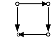
Bases: DiGraphAdapter

A lightweight directed graph implementation optimized for performance and memory efficiency.

This class extends DiGraphAdapter to provide custom storage mechanisms using MapAdapter, which is particularly efficient for graphs with a known, fixed number of nodes.

add_edge(u_of_edge, v_of_edge, **attr)

Add an edge between u and v.

The nodes u and v will be automatically added if they are not already in the graph.

Edge attributes can be specified with keywords or by directly accessing the edge’s attribute dictionary. See examples below.

Parameters:

• u_of_edge (nodes) – Nodes can be, for example, strings or numbers. Nodes must be hashable (and not None) Python objects.

• v_of_edge (nodes) – Nodes can be, for example, strings or numbers. Nodes must be hashable (and not None) Python objects.

• attr (keyword arguments, optional) – Edge data (or labels or objects) can be assigned using keyword arguments.

See also

add_edges_from

add a collection of edges

Notes

Adding an edge that already exists updates the edge data.

Many NetworkX algorithms designed for weighted graphs use an edge attribute (by default weight) to hold a numerical value.

Examples

The following all add the edge e=(1, 2) to graph G:

>>> G = nx.Graph()  # or DiGraph, MultiGraph, MultiDiGraph, etc
>>> e = (1, 2)
>>> G.add_edge(1, 2)  # explicit two-node form
>>> G.add_edge(*e)  # single edge as tuple of two nodes
>>> G.add_edges_from([(1, 2)])  # add edges from iterable container

Associate data to edges using keywords:

>>> G.add_edge(1, 2, weight=3)
>>> G.add_edge(1, 3, weight=7, capacity=15, length=342.7)

For non-string attribute keys, use subscript notation.

>>> G.add_edge(1, 2)
>>> G[1][2].update({0: 5})
>>> G.edges[1, 2].update({0: 5})

add_edges_from(ebunch_to_add, **attr)

Add all the edges in ebunch_to_add.

Parameters:

• ebunch_to_add (container of edges) – Each edge given in the container will be added to the graph. The edges must be given as 2-tuples (u, v) or 3-tuples (u, v, d) where d is a dictionary containing edge data.

• attr (keyword arguments, optional) – Edge data (or labels or objects) can be assigned using keyword arguments.

See also

add_edge

add a single edge

add_weighted_edges_from

convenient way to add weighted edges

Notes

Adding the same edge twice has no effect but any edge data will be updated when each duplicate edge is added.

Edge attributes specified in an ebunch take precedence over attributes specified via keyword arguments.

When adding edges from an iterator over the graph you are changing, a RuntimeError can be raised with message: RuntimeError: dictionary changed size during iteration. This happens when the graph’s underlying dictionary is modified during iteration. To avoid this error, evaluate the iterator into a separate object, e.g. by using list(iterator_of_edges), and pass this object to G.add_edges_from.

Examples

>>> G = nx.Graph()  # or DiGraph, MultiGraph, MultiDiGraph, etc
>>> G.add_edges_from([(0, 1), (1, 2)])  # using a list of edge tuples
>>> e = zip(range(0, 3), range(1, 4))
>>> G.add_edges_from(e)  # Add the path graph 0-1-2-3

Associate data to edges

>>> G.add_edges_from([(1, 2), (2, 3)], weight=3)
>>> G.add_edges_from([(3, 4), (1, 4)], label="WN2898")

Evaluate an iterator over a graph if using it to modify the same graph

>>> G = nx.DiGraph([(1, 2), (2, 3), (3, 4)])
>>> # Grow graph by one new node, adding edges to all existing nodes.
>>> # wrong way - will raise RuntimeError
>>> # G.add_edges_from(((5, n) for n in G.nodes))
>>> # right way - note that there will be no self-edge for node 5
>>> G.add_edges_from(list((5, n) for n in G.nodes))

adjacency()

Returns an iterator over (node, adjacency dict) tuples for all nodes.

For directed graphs, only outgoing neighbors/adjacencies are included.

Returns:

adj_iter – An iterator over (node, adjacency dictionary) for all nodes in the graph.

Return type:

iterator

Examples

>>> G = nx.path_graph(4)  # or DiGraph, MultiGraph, MultiDiGraph, etc
>>> [(n, nbrdict) for n, nbrdict in G.adjacency()]
[(0, {1: {}}), (1, {0: {}, 2: {}}), (2, {1: {}, 3: {}}), (3, {2: {}})]

adjlist_outer_dict_factory() → MapAdapter

Return cheat_adjlist_outer_dict function.

The adjlist_outer_dict_factory method is responsible for creating a factory that produces the outer dictionary for the adjacency list of the TinyDiGraph. In this case, it returns the cheat_adjlist_outer_dict method, which is a custom method designed to create a MapAdapter instance. This MapAdapter serves as a highly efficient, list-based dictionary for storing the adjacency lists of each node in the graph.

The primary purpose of this method is to allow TinyDiGraph to leverage a more memory-efficient data structure for its adjacency list compared to a standard Python dictionary. By using a MapAdapter, the graph can achieve better performance, especially when the number of nodes is known in advance. This method is part of the internal factory customization that allows TinyDiGraph to be optimized for specific use cases.

Returns:

a list-based dictionary for storing node attributes

Return type:

MapAdapter

Examples

>>> graph = TinyDiGraph()
>>> graph.init_nodes(2)
>>> factory = graph.adjlist_outer_dict_factory()
>>> isinstance(factory, MapAdapter)
True

cheat_adjlist_outer_dict() → MapAdapter

Creates a MapAdapter instance to store adjacency lists.

Returns:

A list-based dictionary where nodes store _UNINIT sentinels.

Dicts are allocated lazily on first access — this saves ~232 bytes per node for nodes that never have edges.

Return type:

MapAdapter

Examples

>>> graph = TinyDiGraph()
>>> graph.init_nodes(2)
>>> adj_list = graph.cheat_adjlist_outer_dict()
>>> list(adj_list.keys())
[0, 1]
>>> adj_list[0] is _UNINIT
True

cheat_node_dict() → MapAdapter

Creates a MapAdapter instance to store node attributes.

Returns:

A list-based dictionary where each node’s attributes are stored

in a separate dictionary at the node’s index position.

Return type:

MapAdapter

Examples

>>> graph = TinyDiGraph()
>>> graph.init_nodes(3)
>>> node_dict = graph.cheat_node_dict()
>>> list(node_dict.keys())
[0, 1, 2]
>>> node_dict[0]
{}

get_edge_data(u, v, default=None)

Returns the attribute dictionary associated with edge (u, v).

This is identical to G[u][v] except the default is returned instead of an exception if the edge doesn’t exist.

Parameters:

• u (nodes)

• v (nodes)

• default (any Python object (default=None)) – Value to return if the edge (u, v) is not found.

Returns:

edge_dict – The edge attribute dictionary.

Return type:

dictionary

Examples

>>> G = nx.path_graph(4)  # or DiGraph, MultiGraph, MultiDiGraph, etc
>>> G[0][1]
{}

Warning: Assigning to G[u][v] is not permitted. But it is safe to assign attributes G[u][v][‘foo’]

>>> G[0][1]["weight"] = 7
>>> G[0][1]["weight"]
7
>>> G[1][0]["weight"]
7

>>> G = nx.path_graph(4)  # or DiGraph, MultiGraph, MultiDiGraph, etc
>>> G.get_edge_data(0, 1)  # default edge data is {}
{}
>>> e = (0, 1)
>>> G.get_edge_data(*e)  # tuple form
{}
>>> G.get_edge_data("a", "b", default=0)  # edge not in graph, return 0
0

has_edge(u, v)

Returns True if the edge (u, v) is in the graph.

This is the same as v in G[u] without KeyError exceptions.

Parameters:

• u (nodes) – Nodes can be, for example, strings or numbers. Nodes must be hashable (and not None) Python objects.

• v (nodes) – Nodes can be, for example, strings or numbers. Nodes must be hashable (and not None) Python objects.

Returns:

edge_ind – True if edge is in the graph, False otherwise.

Return type:

bool

Examples

>>> G = nx.path_graph(4)  # or DiGraph, MultiGraph, MultiDiGraph, etc
>>> G.has_edge(0, 1)  # using two nodes
True
>>> e = (0, 1)
>>> G.has_edge(*e)  #  e is a 2-tuple (u, v)
True
>>> e = (0, 1, {"weight": 7})
>>> G.has_edge(*e[:2])  # e is a 3-tuple (u, v, data_dictionary)
True

The following syntax are equivalent:

>>> G.has_edge(0, 1)
True
>>> 1 in G[0]  # though this gives KeyError if 0 not in G
True

in_degree(n=None)

An InDegreeView for (node, in_degree) or in_degree for single node.

The node in_degree is the number of edges pointing to the node. The weighted node degree is the sum of the edge weights for edges incident to that node.

This object provides an iteration over (node, in_degree) as well as lookup for the degree for a single node.

Parameters:

• nbunch (single node, container, or all nodes (default= all nodes)) – The view will only report edges incident to these nodes.

• weight (string or None, optional (default=None)) – The name of an edge attribute that holds the numerical value used as a weight. If None, then each edge has weight 1. The degree is the sum of the edge weights adjacent to the node.

Returns:

• If a single node is requested

• deg (int) – In-degree of the node

• OR if multiple nodes are requested

• nd_iter (iterator) – The iterator returns two-tuples of (node, in-degree).

See also

degree, out_degree

Examples

>>> G = nx.DiGraph()
>>> nx.add_path(G, [0, 1, 2, 3])
>>> G.in_degree(0)  # node 0 with degree 0
0
>>> list(G.in_degree([0, 1, 2]))
[(0, 0), (1, 1), (2, 1)]

init_nodes(num_nodes: int) → None

Initializes the graph with a specified number of nodes.

Sets up the internal data structures for node storage, adjacency lists (successors), and predecessor lists. This method must be called before adding any edges.

Parameters:

num_nodes (int) – The number of nodes to initialize in the graph. Nodes will be indexed from 0 to num_nodes-1.

Examples

>>> graph = TinyDiGraph()
>>> graph.init_nodes(5)
>>> graph.number_of_nodes()
5
>>> list(graph._node.keys())
[0, 1, 2, 3, 4]
>>> list(graph._adj.keys())
[0, 1, 2, 3, 4]

items()

Returns an iterator over (node, adjacency dict) pairs for all nodes.

This method overrides the default items() method to use adjacency() instead, providing a consistent interface for iterating through the graph’s nodes and their connections.

Examples

>>> graph = DiGraphAdapter()
>>> graph.add_edge(1, 2)
>>> graph.add_edge(2, 3)
>>> sorted(list(graph.items()))
[(1, {2: {}}), (2, {3: {}}), (3, {})]

neighbors(n)

Returns an iterator over successor nodes of n.

A successor of n is a node m such that there exists a directed edge from n to m.

Parameters:

n (node) – A node in the graph

Raises:

NetworkXError – If n is not in the graph.

See also

predecessors

Notes

neighbors() and successors() are the same.

node_dict_factory() → MapAdapter

Return cheat_node_dict function.

The node_dict_factory method is responsible for creating a factory that produces the dictionary used to store node attributes in the TinyDiGraph. In this specific implementation, it returns the cheat_node_dict method, which is a custom function designed to create a MapAdapter instance. This MapAdapter serves as a highly efficient, list-based dictionary for storing node attributes.

The primary purpose of this method is to allow TinyDiGraph to leverage a more memory-efficient data structure for its node storage compared to a standard Python dictionary. By using a MapAdapter, the graph can achieve better performance, especially when the number of nodes is known in advance. This method is part of the internal factory customization that allows TinyDiGraph to be optimized for specific use cases.

Returns:

a list-based dictionary for storing node attributes

Return type:

MapAdapter

Examples

>>> graph = TinyDiGraph()
>>> graph.init_nodes(3)
>>> factory = graph.node_dict_factory()
>>> isinstance(factory, MapAdapter)
True

num_nodes = 0

out_degree(n=None)

An OutDegreeView for (node, out_degree)

The node out_degree is the number of edges pointing out of the node. The weighted node degree is the sum of the edge weights for edges incident to that node.

This object provides an iterator over (node, out_degree) as well as lookup for the degree for a single node.

Parameters:

• nbunch (single node, container, or all nodes (default= all nodes)) – The view will only report edges incident to these nodes.

• weight (string or None, optional (default=None)) – The name of an edge attribute that holds the numerical value used as a weight. If None, then each edge has weight 1. The degree is the sum of the edge weights adjacent to the node.

Returns:

• If a single node is requested

• deg (int) – Out-degree of the node

• OR if multiple nodes are requested

• nd_iter (iterator) – The iterator returns two-tuples of (node, out-degree).

See also

degree, in_degree

Examples

>>> G = nx.DiGraph()
>>> nx.add_path(G, [0, 1, 2, 3])
>>> G.out_degree(0)  # node 0 with degree 1
1
>>> list(G.out_degree([0, 1, 2]))
[(0, 1), (1, 1), (2, 1)]

remove_edge(u, v)

Remove the edge between u and v.

Parameters:

• u (nodes) – Remove the edge between nodes u and v.

• v (nodes) – Remove the edge between nodes u and v.

Raises:

NetworkXError – If there is not an edge between u and v.

See also

remove_edges_from

remove a collection of edges

Examples

>>> G = nx.Graph()  # or DiGraph, etc
>>> nx.add_path(G, [0, 1, 2, 3])
>>> G.remove_edge(0, 1)
>>> e = (1, 2)
>>> G.remove_edge(*e)  # unpacks e from an edge tuple
>>> e = (2, 3, {"weight": 7})  # an edge with attribute data
>>> G.remove_edge(*e[:2])  # select first part of edge tuple

successors(n)

Returns an iterator over successor nodes of n.

A successor of n is a node m such that there exists a directed edge from n to m.

Parameters:

n (node) – A node in the graph

Raises:

NetworkXError – If n is not in the graph.

See also

predecessors

Notes

neighbors() and successors() are the same.

Module contents

class digraphx.CSRDiGraph

Bases: Mapping

Memory‑efficient directed graph using Compressed Sparse Row storage.

Nodes must be integers 0 .. N-1. Call init_nodes() first, then add_edge() any number of times, then call freeze() to compact storage. After freezing the graph is still fully readable but no longer supports edge addition.

Examples

>>> g = CSRDiGraph()
>>> g.init_nodes(3)
>>> g.add_edge(0, 1, weight=7)
>>> g.add_edge(1, 2, weight=3)
>>> g.add_edge(2, 0, weight=-5)
>>> g.freeze()
>>> sorted(g[0].items())
[(1, {'weight': 7})]
>>> list(g.nodes())
[0, 1, 2]

add_edge(u: int, v: int, **attr) → None

Add a directed edge u → v with optional attributes.

freeze() → None

Compact internal storage to CSR arrays.

After this call the graph is read‑only.

init_nodes(num_nodes: int) → None

Allocate storage for num_nodes (0 … num_nodes-1).

items() → a set-like object providing a view on D's items

nodes()

Return all node identifiers.

class digraphx.DiGraphAdapter(*args, backend=None, **kwargs)

Bases: DiGraph, MutableMapping

items() → ItemsView

Returns an iterator over (node, adjacency dict) pairs for all nodes.

This method overrides the default items() method to use adjacency() instead, providing a consistent interface for iterating through the graph’s nodes and their connections.

Examples

>>> graph = DiGraphAdapter()
>>> graph.add_edge(1, 2)
>>> graph.add_edge(2, 3)
>>> sorted(list(graph.items()))
[(1, {2: {}}), (2, {3: {}}), (3, {})]

class digraphx.MaxParametricSolver(digraph: Mapping[Node, Mapping[Node, Arc]], omega: ParametricAPI[Node, Arc, Ratio])

Bases: Generic[Node, Arc, Ratio]

Maximum Parametric Solver

This class solves the following parametric network problem:

max r

s.t. dist[v] - dist[u] <= distrance(e, r)

forall e(u, v) in G(V, E)

A parametric network problem refers to a type of optimization problem that involves finding the optimal solution to a network flow problem as a function of one single parameter.

run(dist: MutableMapping[Node, Domain], ratio: Ratio) → Tuple[Ratio, List[Arc]]

The run function takes in a distance mapping and a ratio, and iteratively finds the minimum ratio and corresponding cycle until the minimum ratio is greater than or equal to the input ratio.

Parameters:

• dist (MutableMapping[Node, Domain]) – The dist parameter is a mutable mapping where the keys are Node objects and the values are Domain objects. It represents the distance between nodes in a graph. This distance mapping is updated during the algorithm’s execution.

• ratio (Ratio) – The ratio parameter is a value that represents a ratio or proportion. It is used as a threshold or target value in the algorithm. The algorithm will try to find the maximum possible ratio that satisfies the constraints.

Returns:

The function run returns a tuple containing two elements: 1. The updated ratio (ratio) which is the maximum ratio found that satisfies the constraints 2. The cycle (cycle) that corresponds to this ratio

Return type:

Tuple[Ratio, Cycle]

Examples

>>> from fractions import Fraction
>>> from .min_cycle_ratio import CycleRatioAPI
>>> digraph = {
...     'a': {'b': {'cost': 5, 'time': 1}},
...     'b': {'c': {'cost': 3, 'time': 1}},
...     'c': {'a': {'cost': -2, 'time': 1}}
... }
>>> omega = CycleRatioAPI(digraph, Fraction)
>>> solver = MaxParametricSolver(digraph, omega)
>>> dist = {node: Fraction(0) for node in digraph}
>>> ratio, cycle = solver.run(dist, Fraction(10))
>>> ratio
Fraction(2, 1)

class digraphx.MinCycleRatioSolver(digraph: MutableMapping[Node, Mapping[Node, EdgeType]])

Bases: Generic[Node, EdgeType, Ratio]

Minimum Cycle Ratio Solver

This class solves the following parametric network problem:

max r

s.t. dist[v] - dist[u] <= cost(u, v) - ratio * time(u, v)

for all (u, v) in E

The minimum cycle ratio (MCR) problem is a fundamental problem in the analysis of directed graphs. Given a directed graph, the MCR problem seeks to find the cycle with the minimum ratio of the sum of edge weights to the number of edges in the cycle. In other words, the MCR problem seeks to find the “tightest” cycle in the graph, where the tightness of a cycle is measured by the ratio of the total weight of the cycle to its length.

The MCR problem has many applications in the analysis of discrete event systems, such as digital circuits and communication networks. It is closely related to other problems in graph theory, such as the shortest path problem and the maximum flow problem. Efficient algorithms for solving the MCR problem are therefore of great practical importance.

run(dist: MutableMapping[Node, Domain], ratio0: Ratio) → Tuple[Ratio, List[Arc]]

Run the minimum cycle ratio solver algorithm.

The algorithm works by: 1. Creating a CycleRatioAPI instance with the graph and ratio type 2. Using a MaxParametricSolver to find the optimal ratio 3. Returning both the optimal ratio and the corresponding cycle

Parameters:

• dist (MutableMapping[Node, Domain]) – Initial distance labels for nodes

• ratio0 (Ratio) – Initial ratio value to start the search

Returns:

A tuple containing the optimal ratio and the cycle that achieves it

Return type:

Tuple[Ratio, Cycle]

class digraphx.MinParametricSolver(digraph: Mapping[Node, Mapping[Node, Arc]], omega: MinParametricAPI[Node, Arc, Ratio])

Bases: Generic[Node, Arc, Ratio, Domain]

Minimum Parametric Solver with constraints

This class solves the following parametric network problem:

min r

s.t. dist[v] - dist[u] <= distrance(e, r)

forall e(u, v) in G(V, E)

A parametric network problem refers to a type of optimization problem that involves finding the optimal solution to a network flow problem as a function of one single parameter.

run(dist: MutableMapping[Node, Domain], ratio: Ratio, update_ok: Callable[[Domain, Domain], bool], pick_one_only: bool = False) → Tuple[Ratio, List[Arc]]

The run function executes the parametric solver algorithm to find the minimum ratio.

Parameters:

• dist (MutableMapping[Node, Domain]) – A mutable mapping of node distances that will be updated during the algorithm. Represents the current distance estimates between nodes.

• ratio (Ratio) – The initial ratio value to start the optimization from.

• update_ok (Callable[[Domain, Domain], bool]) – A callback function that determines whether a distance update is acceptable. Takes current and new distance values, returns True if update should proceed.

• pick_one_only (bool) – If True, stops after finding the first improving cycle. Defaults to False.

Returns:

A tuple containing: - The minimum ratio found (ratio) - The cycle that corresponds to this ratio (cycle)

class digraphx.NegCycleFinder(digraph: Mapping[Node, Mapping[Node, Arc]])

Bases: Generic[Node, Arc, Domain]

Negative Cycle Finder by Howard’s method

This code defines a NegCycleFinder class, which is used to find negative cycles in a given directed graph. The NegCycleFinder class has the following methods:

1. __init__(self, digraph: MutableMapping[Node, List[Arc]]): The constructor initializes an instance of the NegCycleFinder class with the given directed graph.

2. relax(self, dist: MutableMapping[Node, Domain], get_weight: Callable[[Arc], Domain]) -> bool: This method performs one iteration of Bellman-Ford algorithm to relax all edges in the graph and update the shortest distances to their neighbors. It returns a boolean value indicating if any changes were made during this iteration.

3. howard(self, dist: MutableMapping[Node, Domain], get_weight: Callable[[Arc], Domain]) -> Generator[Cycle, None, None]: This method finds negative cycles in the graph using the Howard’s algorithm and returns a generator that yields a list of edges for each cycle.

4. cycle_list(self, handle: Node) -> Cycle: This method returns a list of edges that form a cycle in the graph, starting from a given node.

5. is_negative(self, handle: Node, dist: MutableMapping[Node, Domain], get_weight: Callable[[Arc], Domain]) -> bool: This method checks if a cycle is negative by comparing the distances between nodes and the weights of the edges.

Here’s a brief explanation of the algorithms used in this code:

1. Bellman-Ford Algorithm: It is a shortest path algorithm that can find single source shortest paths in a graph with negative edge weights. It runs in O(V*E) time complexity.

2. Howard’s Policy Graph Algorithm: It is used to find cycles in a directed graph and is based on the Bellman-Ford Algorithm. It runs in O(V*E + V*E^2) time complexity in the worst case.

cycle_list(handle: Node) → List[Arc]

Reconstruct the cycle starting from the given node.

Parameters:

handle – The starting node of the cycle (must be part of a cycle)

Returns:

List of edges forming the cycle in order

Return type:

Cycle

Note

Follows predecessor links until returning to the starting node

Examples

>>> digraph = {
...     'a': {'b': 'ab'},
...     'b': {'c': 'bc'},
...     'c': {'a': 'ca'}
... }
>>> finder = NegCycleFinder(digraph)
>>> finder.pred = {'b': ('a', 'ab'), 'c': ('b', 'bc'), 'a': ('c', 'ca')}
>>> finder.cycle_list('a')
['ca', 'bc', 'ab']

find_cycle() → Generator[Node, None, None]

Find cycles in the current predecessor graph using depth-first search.

Yields:

Generator[Node, None, None] –

Each node that starts a cycle in the

predecessor graph

Note

Uses a coloring algorithm (white/gray/black) to detect cycles: - White: unvisited nodes - Gray: nodes being visited in current DFS path - Black: fully visited nodes

Examples

>>> digraph = {
...     "a0": {"a1": 7, "a2": 5},
...     "a1": {"a0": 0, "a2": 3},
...     "a2": {"a1": 1, "a0": 2},
... }
>>> finder = NegCycleFinder(digraph)
>>> for cycle in finder.find_cycle():
...     print(cycle)

howard(dist: MutableMapping[Node, Domain], get_weight: Callable[[Arc], Domain]) → Generator[List[Arc], None, None]

Main algorithm to find negative cycles using Howard’s method.

Parameters:

• dist – Initial distance estimates (often initialized to zero)

• get_weight – Function to get edge weights

Yields:

Generator[Cycle, None, None] – Each found negative cycle as a list of edges

Note

1. Repeatedly relaxes edges until no more improvements can be made

2. Checks for cycles in the predecessor graph

3. Verifies if found cycles are negative

4. Yields each negative cycle found

Examples

>>> digraph = {
...     "a0": {"a1": 7, "a2": 5},
...     "a1": {"a0": 0, "a2": 3},
...     "a2": {"a1": 1, "a0": 2},
... }
>>> dist = {vtx: 0 for vtx in digraph}
>>> finder = NegCycleFinder(digraph)
>>> has_neg = False
>>> for _ in finder.howard(dist, lambda edge: edge):
...     has_neg = True
...     break
...
>>> has_neg
False

is_negative(handle: Node, dist: MutableMapping[Node, Domain], get_weight: Callable[[Arc], Domain]) → bool

Check if the cycle starting at ‘handle’ is negative.

Parameters:

• handle – Starting node of the cycle to check

• dist – Current distance estimates

• get_weight – Function to get edge weights

Returns:

True if the cycle is negative, False otherwise

Return type:

bool

Note

A cycle is negative if the sum of its edge weights is negative. This is checked by verifying that for at least one edge (u,v) in the cycle, dist[v] > dist[u] + weight(u,v) (triangle inequality violation)

Examples

>>> digraph = {
...     'a': {'b': 1},
...     'b': {'c': 1},
...     'c': {'a': -3}
... }
>>> dist = {'a': 0, 'b': 1, 'c': 2}
>>> finder = NegCycleFinder(digraph)
>>> finder.pred = {'b': ('a', 1), 'c': ('b', 1), 'a': ('c', -3)}
>>> finder.is_negative('a', dist, lambda edge: edge)
True

pred: Dict[Node, Tuple[Node, Arc]]

relax(dist: MutableMapping[Node, Domain], get_weight: Callable[[Arc], Domain]) → bool

Perform one relaxation pass of the Bellman-Ford algorithm.

Parameters:

• dist – Current shortest distance estimates for each node

• get_weight – Function to get weight/cost of an edge

Returns:

True if any distance was updated, False otherwise

Return type:

bool

Note

Updates both distance estimates (dist) and predecessor information (pred) for all edges in the graph following the Bellman-Ford relaxation rule: if dist[v] > dist[u] + weight(u,v), then update dist[v]

Examples

>>> digraph = {
...     'a': {'b': 1, 'c': 4},
...     'b': {'c': 2},
...     'c': {'a': -5}
... }
>>> dist = {'a': 0, 'b': float('inf'), 'c': float('inf')}
>>> finder = NegCycleFinder(digraph)
>>> finder.relax(dist, lambda edge: edge)
True
>>> dist['b']
1
>>> dist['c']
3

class digraphx.NegCycleFinderQ(digraph: Mapping[Node, Mapping[Node, Arc]])

Bases: Generic[Node, Arc, Domain]

Negative Cycle Finder with constraints by Howard’s method

Howard’s method is a minimum cycle ratio (MCR) algorithm that uses a policy iteration algorithm to find the minimum cycle ratio of a directed graph. The algorithm maintains a set of candidate cycles and iteratively updates the cycle with the minimum ratio until convergence. To detect negative cycles, Howard’s method uses a cycle detection algorithm that is based on the Bellman-Ford relaxation algorithm. Specifically, the algorithm maintains a predecessor graph of the original graph and performs cycle detection on this graph using the Bellman-Ford relaxation algorithm. If a negative cycle is detected, the algorithm terminates and returns the cycle.

The class implements both predecessor and successor versions of Howard’s algorithm, providing flexibility in how negative cycles are detected and processed.

cycle_list(handle: Node, point_to: Dict[Node, Tuple[Node, Arc]]) → List[Arc]

Reconstruct the cycle starting from the given node.

Parameters:

• handle – Starting node of the cycle

• point_to – Either self.pred or self.succ dictionary defining the edges

Returns:

List of edges forming the cycle in order

Return type:

Cycle

Note

Follows the predecessor/successor links until returning to starting node

Examples

>>> digraph = {
...     'a': {'b': 'ab'},
...     'b': {'c': 'bc'},
...     'c': {'a': 'ca'}
... }
>>> finder = NegCycleFinderQ(digraph)
>>> finder.pred = {'b': ('a', 'ab'), 'c': ('b', 'bc'), 'a': ('c', 'ca')}
>>> finder.cycle_list('a', finder.pred)
['ca', 'bc', 'ab']

find_cycle(point_to: Dict[Node, Tuple[Node, Arc]]) → Generator[Node, None, None]

Detect cycles in the current predecessor/successor graph using depth-first search.

Parameters:

point_to – Either self.pred or self.succ dictionary defining the graph edges

Yields:

Generator[Node, None, None] – Each node that starts a cycle in the graph

Algorithm:

1. Uses a coloring approach (white/gray/black) for cycle detection

2. White nodes are unvisited

3. Gray nodes are currently being visited in DFS stack

4. Black nodes are fully processed

5. A cycle is detected when we encounter a gray node during DFS

Examples

>>> digraph = {
...     "a0": {"a1": 7, "a2": 5},
...     "a1": {"a0": 0, "a2": 3},
...     "a2": {"a1": 1, "a0": 2},
... }
>>> finder = NegCycleFinderQ(digraph)
>>> for cycle in finder.find_cycle(finder.pred):
...     print(cycle)

howard_pred(dist: MutableMapping[Node, Domain], get_weight: Callable[[Arc], Domain], update_ok: Callable[[Domain, Domain], bool]) → Generator[List[Arc], None, None]

Find negative cycles using predecessor-based Howard’s algorithm.

Parameters:

• dist – Initial distance estimates (often zero-initialized)

• get_weight – Function to get weight of an edge

• update_ok – Function to determine if distance updates are allowed

Yields:

Generator[Cycle, None, None] – Each negative cycle found as a list of edges

Algorithm:

1. Repeatedly relax edges using predecessor updates

2. After each relaxation, check for cycles in predecessor graph

3. If cycle found, verify if it’s negative

4. Yield each negative cycle found

Examples

>>> digraph = {
...     "a0": {"a1": 7, "a2": 5},
...     "a1": {"a0": 0, "a2": 3},
...     "a2": {"a1": 1, "a0": 2},
... }
>>> dist = {vtx: 0 for vtx in digraph}
>>> def update_ok(dist, v) : return True
>>> finder = NegCycleFinderQ(digraph)
>>> has_neg = False
>>> for _ in finder.howard_pred(dist, lambda edge: edge, update_ok):
...     has_neg = True
...     break
...
>>> has_neg
False

howard_succ(dist: MutableMapping[Node, Domain], get_weight: Callable[[Arc], Domain], update_ok: Callable[[Domain, Domain], bool]) → Generator[List[Arc], None, None]

Find negative cycles using successor-based Howard’s algorithm.

Parameters:

• dist – Initial distance estimates (often zero-initialized)

• get_weight – Function to get weight of an edge

• update_ok – Function to determine if distance updates are allowed

Yields:

Generator[Cycle, None, None] – Each negative cycle found as a list of edges

Note

Similar to howard_pred but uses successor updates instead of predecessor Currently skips the negative cycle verification (commented assert)

Examples

>>> digraph = {
...     "a0": {"a1": 7, "a2": 5},
...     "a1": {"a0": 0, "a2": 3},
...     "a2": {"a1": 1, "a0": 2},
... }
>>> def update_ok(dist, v) : return True
>>> dist = {vtx: 0 for vtx in digraph}
>>> finder = NegCycleFinderQ(digraph)
>>> has_neg = False
>>> for _ in finder.howard_succ(dist, lambda edge: edge, update_ok):
...     has_neg = True
...     break
...
>>> has_neg
False

is_negative(handle: Node, dist: MutableMapping[Node, Domain], get_weight: Callable[[Arc], Domain]) → bool

Verify if the cycle starting at handle is negative.

Parameters:

• handle – Starting node of the cycle

• dist – Current distance estimates

• get_weight – Function to get weight of an edge

Returns:

True if the cycle is negative, False otherwise

Return type:

bool

Note

A cycle is negative if the sum of its edge weights is negative This is detected by finding at least one edge that violates the triangle inequality: dist[v] > dist[u] + weight(u,v)

Examples

>>> digraph = {
...     'a': {'b': 1},
...     'b': {'c': 1},
...     'c': {'a': -3}
... }
>>> dist = {'a': 0, 'b': 1, 'c': 2}
>>> finder = NegCycleFinderQ(digraph)
>>> finder.pred = {'b': ('a', 1), 'c': ('b', 1), 'a': ('c', -3)}
>>> finder.is_negative('a', dist, lambda edge: edge)
True

pred: Dict[Node, Tuple[Node, Arc]]

relax_pred(dist: MutableMapping[Node, Domain], get_weight: Callable[[Arc], Domain], update_ok: Callable[[Domain, Domain], bool]) → bool

Perform predecessor relaxation step (Bellman-Ford style).

Parameters:

• dist – Current distance estimates for each node

• get_weight – Function to get weight of an edge

• update_ok – Function to determine if distance update should be applied

Returns:

True if any distances were updated, False otherwise

Return type:

bool

Note

Updates distances based on predecessor edges (u -> v) Implements the relaxation: if dist[v] > dist[u] + weight(u,v), update dist[v]

Examples

>>> digraph = {
...     'a': {'b': 1, 'c': 4},
...     'b': {'c': 2},
...     'c': {'a': -5}
... }
>>> dist = {'a': 0, 'b': float('inf'), 'c': float('inf')}
>>> finder = NegCycleFinderQ(digraph)
>>> finder.relax_pred(dist, lambda edge: edge, lambda old, new: True)
True
>>> dist['b']
1
>>> dist['c']
3

relax_succ(dist: MutableMapping[Node, Domain], get_weight: Callable[[Arc], Domain], update_ok: Callable[[Domain, Domain], bool]) → bool

Perform successor relaxation step (reverse Bellman-Ford style).

Parameters:

• dist – Current distance estimates for each node

• get_weight – Function to get weight of an edge

• update_ok – Function to determine if distance update should be applied

Returns:

True if any distances were updated, False otherwise

Return type:

bool

Note

Updates distances based on successor edges (u -> v) Implements the relaxation: if dist[u] < dist[v] - weight(u,v), update dist[u]

Examples

>>> digraph = {
...     'a': {'b': 1},
...     'b': {}
... }
>>> dist = {'a': 0, 'b': 5}
>>> finder = NegCycleFinderQ(digraph)
>>> finder.relax_succ(dist, lambda edge: edge, lambda old, new: True)
True
>>> dist['a']
4

succ: Dict[Node, Tuple[Node, Arc]]

class digraphx.TinyDiGraph(*args, backend=None, **kwargs)

Bases: DiGraphAdapter

A lightweight directed graph implementation optimized for performance and memory efficiency.

This class extends DiGraphAdapter to provide custom storage mechanisms using MapAdapter, which is particularly efficient for graphs with a known, fixed number of nodes.

add_edge(u_of_edge, v_of_edge, **attr)

Add an edge between u and v.

The nodes u and v will be automatically added if they are not already in the graph.

Edge attributes can be specified with keywords or by directly accessing the edge’s attribute dictionary. See examples below.

Parameters:

• u_of_edge (nodes) – Nodes can be, for example, strings or numbers. Nodes must be hashable (and not None) Python objects.

• v_of_edge (nodes) – Nodes can be, for example, strings or numbers. Nodes must be hashable (and not None) Python objects.

• attr (keyword arguments, optional) – Edge data (or labels or objects) can be assigned using keyword arguments.

See also

add_edges_from

add a collection of edges

Notes

Adding an edge that already exists updates the edge data.

Many NetworkX algorithms designed for weighted graphs use an edge attribute (by default weight) to hold a numerical value.

Examples

The following all add the edge e=(1, 2) to graph G:

>>> G = nx.Graph()  # or DiGraph, MultiGraph, MultiDiGraph, etc
>>> e = (1, 2)
>>> G.add_edge(1, 2)  # explicit two-node form
>>> G.add_edge(*e)  # single edge as tuple of two nodes
>>> G.add_edges_from([(1, 2)])  # add edges from iterable container

Associate data to edges using keywords:

>>> G.add_edge(1, 2, weight=3)
>>> G.add_edge(1, 3, weight=7, capacity=15, length=342.7)

For non-string attribute keys, use subscript notation.

>>> G.add_edge(1, 2)
>>> G[1][2].update({0: 5})
>>> G.edges[1, 2].update({0: 5})

add_edges_from(ebunch_to_add, **attr)

Add all the edges in ebunch_to_add.

Parameters:

• ebunch_to_add (container of edges) – Each edge given in the container will be added to the graph. The edges must be given as 2-tuples (u, v) or 3-tuples (u, v, d) where d is a dictionary containing edge data.

• attr (keyword arguments, optional) – Edge data (or labels or objects) can be assigned using keyword arguments.

See also

add_edge

add a single edge

add_weighted_edges_from

convenient way to add weighted edges

Notes

Adding the same edge twice has no effect but any edge data will be updated when each duplicate edge is added.

Edge attributes specified in an ebunch take precedence over attributes specified via keyword arguments.

When adding edges from an iterator over the graph you are changing, a RuntimeError can be raised with message: RuntimeError: dictionary changed size during iteration. This happens when the graph’s underlying dictionary is modified during iteration. To avoid this error, evaluate the iterator into a separate object, e.g. by using list(iterator_of_edges), and pass this object to G.add_edges_from.

Examples

>>> G = nx.Graph()  # or DiGraph, MultiGraph, MultiDiGraph, etc
>>> G.add_edges_from([(0, 1), (1, 2)])  # using a list of edge tuples
>>> e = zip(range(0, 3), range(1, 4))
>>> G.add_edges_from(e)  # Add the path graph 0-1-2-3

Associate data to edges

>>> G.add_edges_from([(1, 2), (2, 3)], weight=3)
>>> G.add_edges_from([(3, 4), (1, 4)], label="WN2898")

Evaluate an iterator over a graph if using it to modify the same graph

>>> G = nx.DiGraph([(1, 2), (2, 3), (3, 4)])
>>> # Grow graph by one new node, adding edges to all existing nodes.
>>> # wrong way - will raise RuntimeError
>>> # G.add_edges_from(((5, n) for n in G.nodes))
>>> # right way - note that there will be no self-edge for node 5
>>> G.add_edges_from(list((5, n) for n in G.nodes))

adjacency()

Returns an iterator over (node, adjacency dict) tuples for all nodes.

For directed graphs, only outgoing neighbors/adjacencies are included.

Returns:

adj_iter – An iterator over (node, adjacency dictionary) for all nodes in the graph.

Return type:

iterator

Examples

>>> G = nx.path_graph(4)  # or DiGraph, MultiGraph, MultiDiGraph, etc
>>> [(n, nbrdict) for n, nbrdict in G.adjacency()]
[(0, {1: {}}), (1, {0: {}, 2: {}}), (2, {1: {}, 3: {}}), (3, {2: {}})]

adjlist_outer_dict_factory() → MapAdapter

Return cheat_adjlist_outer_dict function.

The adjlist_outer_dict_factory method is responsible for creating a factory that produces the outer dictionary for the adjacency list of the TinyDiGraph. In this case, it returns the cheat_adjlist_outer_dict method, which is a custom method designed to create a MapAdapter instance. This MapAdapter serves as a highly efficient, list-based dictionary for storing the adjacency lists of each node in the graph.

The primary purpose of this method is to allow TinyDiGraph to leverage a more memory-efficient data structure for its adjacency list compared to a standard Python dictionary. By using a MapAdapter, the graph can achieve better performance, especially when the number of nodes is known in advance. This method is part of the internal factory customization that allows TinyDiGraph to be optimized for specific use cases.

Returns:

a list-based dictionary for storing node attributes

Return type:

MapAdapter

Examples

>>> graph = TinyDiGraph()
>>> graph.init_nodes(2)
>>> factory = graph.adjlist_outer_dict_factory()
>>> isinstance(factory, MapAdapter)
True

cheat_adjlist_outer_dict() → MapAdapter

Creates a MapAdapter instance to store adjacency lists.

Returns:

A list-based dictionary where nodes store _UNINIT sentinels.

Dicts are allocated lazily on first access — this saves ~232 bytes per node for nodes that never have edges.

Return type:

MapAdapter

Examples

>>> graph = TinyDiGraph()
>>> graph.init_nodes(2)
>>> adj_list = graph.cheat_adjlist_outer_dict()
>>> list(adj_list.keys())
[0, 1]
>>> adj_list[0] is _UNINIT
True

cheat_node_dict() → MapAdapter

Creates a MapAdapter instance to store node attributes.

Returns:

A list-based dictionary where each node’s attributes are stored

in a separate dictionary at the node’s index position.

Return type:

MapAdapter

Examples

>>> graph = TinyDiGraph()
>>> graph.init_nodes(3)
>>> node_dict = graph.cheat_node_dict()
>>> list(node_dict.keys())
[0, 1, 2]
>>> node_dict[0]
{}

get_edge_data(u, v, default=None)

Returns the attribute dictionary associated with edge (u, v).

This is identical to G[u][v] except the default is returned instead of an exception if the edge doesn’t exist.

Parameters:

• u (nodes)

• v (nodes)

• default (any Python object (default=None)) – Value to return if the edge (u, v) is not found.

Returns:

edge_dict – The edge attribute dictionary.

Return type:

dictionary

Examples

>>> G = nx.path_graph(4)  # or DiGraph, MultiGraph, MultiDiGraph, etc
>>> G[0][1]
{}

Warning: Assigning to G[u][v] is not permitted. But it is safe to assign attributes G[u][v][‘foo’]

>>> G[0][1]["weight"] = 7
>>> G[0][1]["weight"]
7
>>> G[1][0]["weight"]
7

>>> G = nx.path_graph(4)  # or DiGraph, MultiGraph, MultiDiGraph, etc
>>> G.get_edge_data(0, 1)  # default edge data is {}
{}
>>> e = (0, 1)
>>> G.get_edge_data(*e)  # tuple form
{}
>>> G.get_edge_data("a", "b", default=0)  # edge not in graph, return 0
0

has_edge(u, v)

Returns True if the edge (u, v) is in the graph.

This is the same as v in G[u] without KeyError exceptions.

Parameters:

• u (nodes) – Nodes can be, for example, strings or numbers. Nodes must be hashable (and not None) Python objects.

• v (nodes) – Nodes can be, for example, strings or numbers. Nodes must be hashable (and not None) Python objects.

Returns:

edge_ind – True if edge is in the graph, False otherwise.

Return type:

bool

Examples

>>> G = nx.path_graph(4)  # or DiGraph, MultiGraph, MultiDiGraph, etc
>>> G.has_edge(0, 1)  # using two nodes
True
>>> e = (0, 1)
>>> G.has_edge(*e)  #  e is a 2-tuple (u, v)
True
>>> e = (0, 1, {"weight": 7})
>>> G.has_edge(*e[:2])  # e is a 3-tuple (u, v, data_dictionary)
True

The following syntax are equivalent:

>>> G.has_edge(0, 1)
True
>>> 1 in G[0]  # though this gives KeyError if 0 not in G
True

in_degree(n=None)

An InDegreeView for (node, in_degree) or in_degree for single node.

The node in_degree is the number of edges pointing to the node. The weighted node degree is the sum of the edge weights for edges incident to that node.

This object provides an iteration over (node, in_degree) as well as lookup for the degree for a single node.

Parameters:

• nbunch (single node, container, or all nodes (default= all nodes)) – The view will only report edges incident to these nodes.

• weight (string or None, optional (default=None)) – The name of an edge attribute that holds the numerical value used as a weight. If None, then each edge has weight 1. The degree is the sum of the edge weights adjacent to the node.

Returns:

• If a single node is requested

• deg (int) – In-degree of the node

• OR if multiple nodes are requested

• nd_iter (iterator) – The iterator returns two-tuples of (node, in-degree).

See also

degree, out_degree

Examples

>>> G = nx.DiGraph()
>>> nx.add_path(G, [0, 1, 2, 3])
>>> G.in_degree(0)  # node 0 with degree 0
0
>>> list(G.in_degree([0, 1, 2]))
[(0, 0), (1, 1), (2, 1)]

init_nodes(num_nodes: int) → None

Initializes the graph with a specified number of nodes.

Sets up the internal data structures for node storage, adjacency lists (successors), and predecessor lists. This method must be called before adding any edges.

Parameters:

num_nodes (int) – The number of nodes to initialize in the graph. Nodes will be indexed from 0 to num_nodes-1.

Examples

>>> graph = TinyDiGraph()
>>> graph.init_nodes(5)
>>> graph.number_of_nodes()
5
>>> list(graph._node.keys())
[0, 1, 2, 3, 4]
>>> list(graph._adj.keys())
[0, 1, 2, 3, 4]

items()

Returns an iterator over (node, adjacency dict) pairs for all nodes.

This method overrides the default items() method to use adjacency() instead, providing a consistent interface for iterating through the graph’s nodes and their connections.

Examples

>>> graph = DiGraphAdapter()
>>> graph.add_edge(1, 2)
>>> graph.add_edge(2, 3)
>>> sorted(list(graph.items()))
[(1, {2: {}}), (2, {3: {}}), (3, {})]

neighbors(n)

Returns an iterator over successor nodes of n.

A successor of n is a node m such that there exists a directed edge from n to m.

Parameters:

n (node) – A node in the graph

Raises:

NetworkXError – If n is not in the graph.

See also

predecessors

Notes

neighbors() and successors() are the same.

node_dict_factory() → MapAdapter

Return cheat_node_dict function.

The node_dict_factory method is responsible for creating a factory that produces the dictionary used to store node attributes in the TinyDiGraph. In this specific implementation, it returns the cheat_node_dict method, which is a custom function designed to create a MapAdapter instance. This MapAdapter serves as a highly efficient, list-based dictionary for storing node attributes.

The primary purpose of this method is to allow TinyDiGraph to leverage a more memory-efficient data structure for its node storage compared to a standard Python dictionary. By using a MapAdapter, the graph can achieve better performance, especially when the number of nodes is known in advance. This method is part of the internal factory customization that allows TinyDiGraph to be optimized for specific use cases.

Returns:

a list-based dictionary for storing node attributes

Return type:

MapAdapter

Examples

>>> graph = TinyDiGraph()
>>> graph.init_nodes(3)
>>> factory = graph.node_dict_factory()
>>> isinstance(factory, MapAdapter)
True

num_nodes = 0

out_degree(n=None)

An OutDegreeView for (node, out_degree)

The node out_degree is the number of edges pointing out of the node. The weighted node degree is the sum of the edge weights for edges incident to that node.

This object provides an iterator over (node, out_degree) as well as lookup for the degree for a single node.

Parameters:

• nbunch (single node, container, or all nodes (default= all nodes)) – The view will only report edges incident to these nodes.

• weight (string or None, optional (default=None)) – The name of an edge attribute that holds the numerical value used as a weight. If None, then each edge has weight 1. The degree is the sum of the edge weights adjacent to the node.

Returns:

• If a single node is requested

• deg (int) – Out-degree of the node

• OR if multiple nodes are requested

• nd_iter (iterator) – The iterator returns two-tuples of (node, out-degree).

See also

degree, in_degree

Examples

>>> G = nx.DiGraph()
>>> nx.add_path(G, [0, 1, 2, 3])
>>> G.out_degree(0)  # node 0 with degree 1
1
>>> list(G.out_degree([0, 1, 2]))
[(0, 1), (1, 1), (2, 1)]

remove_edge(u, v)

Remove the edge between u and v.

Parameters:

• u (nodes) – Remove the edge between nodes u and v.

• v (nodes) – Remove the edge between nodes u and v.

Raises:

NetworkXError – If there is not an edge between u and v.

See also

remove_edges_from

remove a collection of edges

Examples

>>> G = nx.Graph()  # or DiGraph, etc
>>> nx.add_path(G, [0, 1, 2, 3])
>>> G.remove_edge(0, 1)
>>> e = (1, 2)
>>> G.remove_edge(*e)  # unpacks e from an edge tuple
>>> e = (2, 3, {"weight": 7})  # an edge with attribute data
>>> G.remove_edge(*e[:2])  # select first part of edge tuple

successors(n)

Returns an iterator over successor nodes of n.

A successor of n is a node m such that there exists a directed edge from n to m.

Parameters:

n (node) – A node in the graph

Raises:

NetworkXError – If n is not in the graph.

See also

predecessors

Notes

neighbors() and successors() are the same.

digraphx.cycle_canceling_mcf(g, demands, sink=None)

Solve min-cost flow using cycle-cancellation descent.

Uses Bellman-Ford for negative-cycle detection (no Howard gap). Optional vertex-disjoint constraint via VertexFilter.

Parameters:

• g – {u: {v: {‘weight’: cost, ‘capacity’: cap}}}

• demands – {node: demand} (negative = supply, positive = demand)

• sink – Optional sink node. When provided, enables the vertex-disjoint constraint: each non-sink node may have at most one outgoing flow edge. When None (default), no constraint is enforced.

Returns:

(total_cost, flow_dict) or None if infeasible.